17 Abstract Machines
So far in this class we have focused on the extensional behavior of programs, or how programs behave "from the outside" by interacting with them. In our next topic we will dive deeper into the intensional behavior of programs and study the behavior of programs as they run. It is very useful to know what a program does, but it is also very useful to know how it does it. Programmers have many questions of this form, like "how long does my program take to run?", "how much memory does my program use as it runs?", or "does this compiler optimization make my programs faster?" These kinds of properties are intensional properties.
To study intensional behavior of programs, we will need a model of the machine that they run on. For this, we will use state machines, sometimes also called abstract machines. These state-machine-based runtime semantics of programs are critical for understanding how expensive programs are to run and give us another vantage point for understanding language implementation strategies, compare languages, and implement programming languages efficiently.
17.1 State Machines
A state machine, sometimes also called a transition system, consists of the following pieces:
A set of states S that the machine can be in.
An initial state that the machine starts in.
A set of final (also called accepting) states F that the machine ends in.
A transition function T : S -> S that describe how the machine evolves over time.
There are a few key differences between your computer and a state machine. Your computer runs forever waiting for your input, so it doesn’t really have a final state. Additionally, your computer does things in parallel, so the transition function seems more complicated. The state machine analogy is a useful abstraction that eliminates these intricacies, so we use it, but it is not perfect.
There are two main ways of describing state machines: using tables and using diagrams. Let’s see both ways.
Suppose we want to design a state machine that makes change: given some total dollar amount, it will tell you how many quarters, dimes, nickels, and pennies you can form out of that total. Here is a diagramatic depiction of this state machine’s transition function:
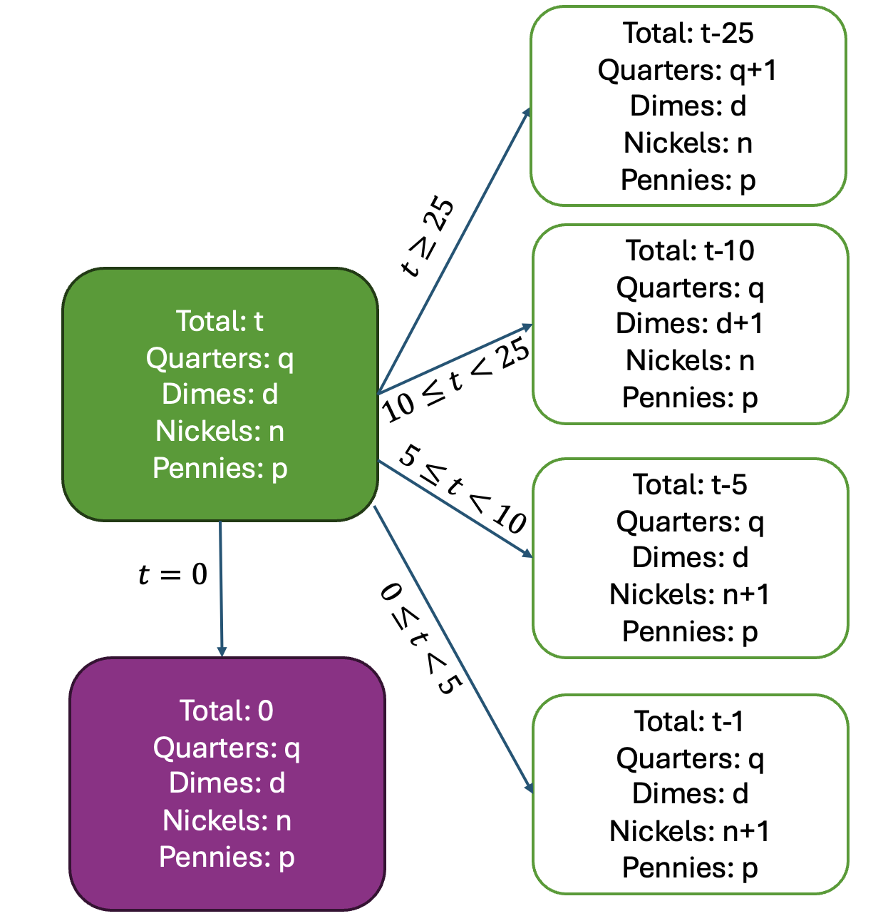
The initial state is shown in green, and the final state in shown in purple. Each state tracks the remaining total dollar ammount and the total amount of change that has been dispensed. Each transition arrow is labeled with a condition that checks the total; in this language of state machines, we permit guarding transition arrows with conditional expressions about the current state. For the transition function to be valid, there must be exactly 1 valid transition arrow for a particular state.
We can represent this same state machine using a table with 4 columns: the current state, the next state, the condition that guards this transition, and whether or not the state is final. The state is written here as (T, Q, D, N, P) where T is the total, Q is the number of quarters, N is the number of nickels, D is the number of dimes, and P is the number of pennies:
Current State |
| Next State |
| Guard |
| Final? |
(T, Q, D, N, P) |
| (T-25, Q+1, D, N, P) |
| T >= 25 |
| N |
(T, Q, N, D, P) |
| (T-10, Q, D+1, N, P) |
| 10 <= T < 25 |
| N |
(T, Q, D, N, P) |
| (T-5, Q, D, N+1, P) |
| 5 <= T < 10 |
| N |
(T, Q, D, N, P) |
| (T-1, Q, D, N, P+1) |
| 0 < T < 5 |
| N |
(T, Q, D, N, P) |
| (T, Q, D, N, P) |
| T = 0 |
| Y |
Once a state machine is defined we can simulate it by picking a state and applying a transition function until a final state is reachede.
We can easily implement the state machine for making change in Plait, where we encode the final state as transitioning to itself:
> (define-type ChangeState (change-state [T : Number] [Q : Number] [D : Number] [N : Number] [P : Number]))
> (define (transition s) (type-case ChangeState s [(change-state T Q D N P) (cond [(>= T 25) (change-state (- T 25) (+ 1 Q) D N P)] [(and (< T 25) (>= T 10)) (change-state (- T 10) Q (+ 1 D) N P)] [(and (< T 10) (>= T 5)) (change-state (- T 5) Q D (+ 1 N) P)] [(and (< T 5) (> T 0)) (change-state (- T 1) Q D N (+ 1 P))] [(equal? T 0) s])]))
> (define (simulate s) (let [(next-state (transition s))] (if (equal? next-state s) s (begin (display s) (display "\n") (simulate next-state))))) > (simulate (change-state 34 0 0 0 0))
- ChangeState
#(struct:change-state 34 0 0 0 0)
#(struct:change-state 9 1 0 0 0)
#(struct:change-state 4 1 0 1 0)
#(struct:change-state 3 1 0 1 1)
#(struct:change-state 2 1 0 1 2)
#(struct:change-state 1 1 0 1 3)
(change-state 0 1 0 1 4)
We can think of the change machine state ChangeState as a simple computer with 5 registers that encode the state of the machine. Each of these registers holds numbers, and we can perform the usual number operations on them (adding, subtracting, comparing). This is not too different from the CPU that runs your computer, which is a Von Neumann-style CPU with registers for arithmetic, a control register, etc.
17.2 The CK Machine
The CC, CK, CEK, and CESK machines are from Matthias Felleisen’s PhD. thesis. Since then they have become quite widespread tools for describing the intensional behavior of programs.
Now let’s design a state machine for running programs, sometimes also called a central processing unit (CPU). We will implement this CPU in Plait: this implementatin will be called a abstract machine. As usual, we start with the simplest smallest language, Calc:
> (define-type Calc (addE [e1 : Calc] [e2 : Calc]) (numE [n : Number]))
Different choices of representing the state of the abstract machine will yield different kinds of machines with different runtime behavior. The first machine we will study is the CK machine, whose state consists of two components:
The control register C, which is the current instruction.
The stacK register K that holds a representation of the call stack.
If you like, you can magine that of the control register as containing a pointer to a Calc abstract syntax datastructure, so that it behaves and looks more like a typical instruction pointer on your CPU.
We want to perform this recursive computation using a our state machine. To do this, we need to keep track of some extra data in the stacK register: in particular, we need to store the frame (also called a call site) that tracks the state of the program when we jump to evaluating the subexpression, so that we know how to resume computation once that subexpression is done.
add1E: An addition (n e2) where n is a number. In this case we need to recursively evaluate e2 and store n so that we can return to it later to finish summing.
add2E: An addition (+ e1 e2) where neither e1 nor e2 are numbers. In this case, we need to recursively evaluate e1, so the callsite needs to store e2 so we can return to finish evaluating it later.
We can represent these two kinds of frames using a Plait datastructure:
> (define-type Frame (add1E [n : Number]) (add2E [e : Calc]))
To handle nested recursion so that we can evaluate expressions like (+ (+ (+ 1 2) 3) 4), our abstract machine will need to maintain a stack of frames, which we represent as a list. This stack is often called the call stack. The state of the CK machine can now be defined as follows:
> (define-type State (state [C : Calc] [K : (Listof Frame)]))
I.e., the state is a pair consisting of (1) a (pointer to the) point in the program that is currently being evaluated, and (2) a call-stack.
17.2.1 Designing the Transition Function
Now we are ready to design the transition function for the CK machine. Here is its complete description as a table:
Current C
Current K
Guard
Next C
Next K
Final?
(addE e1 e2)
K
e1 = n1, e2 = n2
(numE (+ n1 n2))
K
N
(addE e1 e2)
K
e1 not a number
e1
(cons (add2E e2) K)
N
(addE e1 e2)
K
e1 = n1
e2
(cons (add1E n1) K)
N
(numE n)
(cons (add1E n1) K)
K not empty
(addE (numE n) (numE n1))
K
N
(numE n)
(cons (add2E e2) K)
K not empty
(addE (numE n) e2)
K
N
(numE n)
K
K empty
(numE n)
K
Y
Take a moment to carefully examine these rules, and think about what might break if you change any part of the rules. Let’s examine them one by one:
The first rule reduces an addition to a nubmer. The call stack is not changed because no recursive calls are performed and no control is transferred.
The second rule recursively evaluates e1. It pushes an add2E frame onto the stack to remember to jump back to finish evluating e2.
The third rule recursively evaluatse e2 once e1 is a number. It stores the number in a frame.
The fourth and fifth rules implement a "return" construct: they pop the call stack and place the number into the control.
The final rule is the terminating state: programs should halt when there is an empty call stack and a number in the control register.
Here is an example of running the machine according to these rules:
Step #
C
K
1
(addE (addE (numE 1) (numE 2)) (numE 3))
empty
2
(addE (numE 1) (numE 2))
(list (add2E (numE 3)))
2
(numE 3)
(list (add2E (numE 3)))
3
(addE (numE 3) (numE 3))
empty
4
(numE 6)
empty
Figure 26: An example of running a CK machine on the program (+ (+ 1 2) 3)
Once you understand the machine it is relatively easy to implement. Here is a link to a full implementation of the CK machine in Plait.
17.3 Control Flow
Our representation of the above state machine makes the evaluation context explicit. Again, just like when we were studying continuation-passing style, this enables us to implement control-flow operators quite straightforwardly. Let’s extend our grammar with a return construct:
(define-type CalcRet (addE [e1 : CalcRet] [e2 : CalcRet]) (numE [n : Number]) (returnE [n : Number]))
Now, to implement it, we need to add it to our transition function:
Current C
Current K
Guard
Next C
Next K
Final?
(addE e1 e2)
K
e1 = n1, e2 = n2
(numE (+ n1 n2))
K
N
(addE e1 e2)
K
e1 not a number
e1
(cons (add2E e2) K)
N
(addE e1 e2)
K
e1 = n1
e2
(cons (add1E n1) K)
N
(returnE n)
K
(numE n)
empty
N
(numE n)
(cons (add1E n1) K)
K not empty
(addE (numE n) (numE n1))
K
N
(numE n)
(cons (add2E e2) K)
K not empty
(addE (numE n) e2)
K
N
(numE n)
K
K empty
(numE n)
K
Y
Figure 27: A tabular representation of the CK machine for CalcRet.