16 Control Formalism II🔗

Last time we saw how to use evaluation contexts to define the small-step semantics of control flow operators like return. Today we will revisit this topic to explore how to define the small step semantics of exceptions. Along the way, we will revisit the evaluation contexts formalism to clean it up a bit and make it easier to reason about.

16.1 Unique Decompositions🔗

Recall from last time that we defined a notion of an evaluation context E that represents the fragment of the program that an expression is being evaluated in. We defined E as a "program with a hole in it", where the hole is where computation occurrs. In order to implement small step semantics of control operators it’s extremely useful to know exactly which evaluation context an expression is to be evaluated in.

Last time we saw that there was more than 1 evaluation context for a given term. This is quite annoying and undesirable, and it was actually not intentional; let’s fix this!

Recall our tiny language CalcRet from last time and its evaluation contexts:

	‹e›	::=	( + ‹e› ‹e› )
		|	‹num›
		|	( return ‹num› )

Figure 21: Surface syntax for CalcRet.

	‹E›	::=	[.]
		|	( + ‹num› ‹E› )
		|	( + ‹E› ‹e› )

Figure 22: Evaluation context grammar for CalcRet.

Further recall that we defined the syntax E[e] to mean "substitute in the expression e for the hole in E". Now let’s define our small-step semantics, which will be different from last time:

The small-step semantics in the above figure identify our reducible expressions (sometimes abbreviated as "redexes"): expressions that are ready to take a step of computation. The reducible expressions are in the holes: they are addition of numbers (+ n1 n2) and return expression (return n). We can write down a grammar for the reducible expressions that we label as e_{\rightarrow}:

e_{\rightarrow} ::= \texttt{(+ n1 n2)} \mid \texttt{(return n)}

Now we can state our desired property:

Theorem: (Uniqueness of Decomposition) Let e be a CalcLang program and suppose e \rightarrow e{}’. Then, there exists a unique evaluation context E and reducible expression e{}’ where e = E[e{}’].

To prove this fact, we’ll write down another grammar called E[e_{\rightarrow}] that is the set of evaluation contexts with reducible expressions in the holes. Let’s define this grammar:

E[e_\rightarrow] ::= \underbrace{e_{\rightarrow}}_{(1)} \mid \underbrace{(+~E[e_\rightarrow]~e)}_{(2)} \mid \underbrace{(+~\texttt{n}~E[e_\rightarrow])}_{(3)}

Before we establish these facts let’s see some examples of parsing programs using the E[e_{\rightarrow}] grammar:

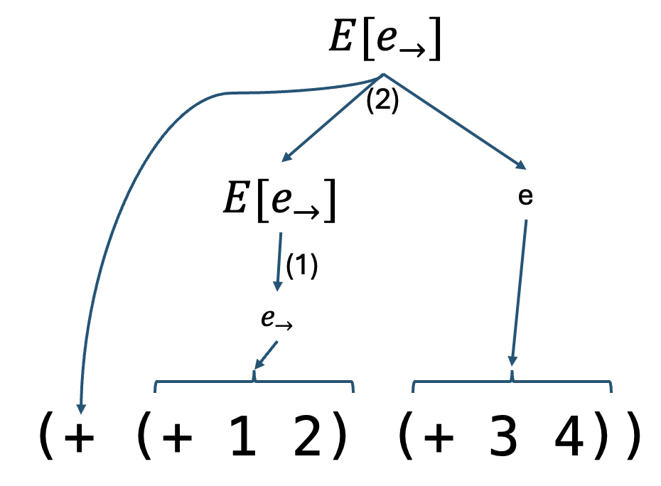
From the above parse tree we can conclude that the unique evaluation context is E1 = (+ [.] (+ 3 4))and e1 = (+ 1 2) is the redex.

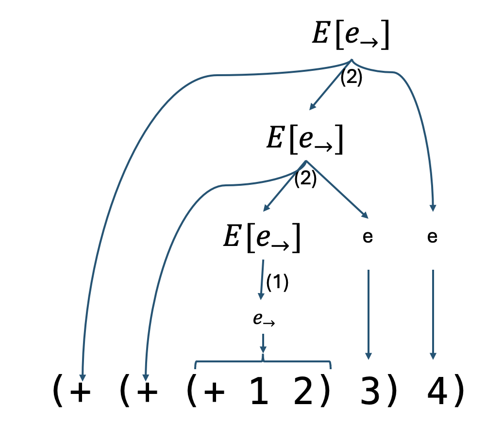
From the above parse tree we can conclude that the unique evaluation context is E2 = (+ (+ [.] 3) 4) and e1 = (+ 1 2) is the redex.

Notice what’s happening when we parse programs using this grammar: by parsing the program, we identify the evaluation context E and the hole [\cdot]. From this tree we can extract an evaluation context E by replacing the focus with the hole [\cdot].

Using these properties we can now prove the uniqueness of decomposition:

Proof of uniqueness of decomposition. By assumption we know e \rightarrow e{}’. This means either the (E-Add) rule or the (E-Ret) rule was applied. In either case, this implies e can be parsed using the E[e_\rightarrow] grammar. By the fact that the grammar is unambiguous and there is at most 1 redex position, this means that there is a unique parse tree that identifies a unique context E where the hole is at the hole position in the parsre tree of E[e_{\rightarrow}].

16.2 Derivation Trees🔗

Phew! That was a lot of work, but there’s a real payoff: now we can always immediately identify the reducible expression and its (unique!) context by parsing a program using the E[e_\rightarrow] grammar. This is very powerful, since it lets us immediately "focus in on" the reducible expression and write down semantics that manipulate the outer context. This is a powerful tool for describing control-flow operators.

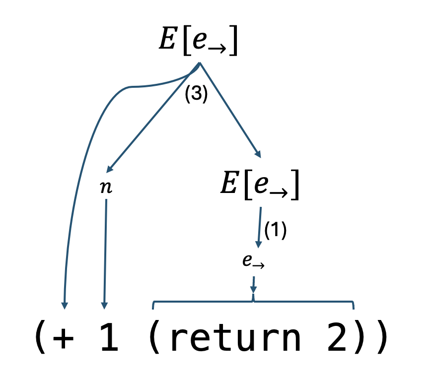
So, from this parsetree we can conclude that E = (+ 1 [.]) and e = (return 2). Now we can apply our E-Add rule:

\dfrac{~}{\texttt{(+ 1 [return 2])}\rightarrow 2}~\text{(E-Add)}

And we see this program runs to 2.

16.3 Semantics of Exceptions🔗

Now let’s see the power of the formalism by extending the untyped lambda calculus with exceptions.

Here is the semantics, where we use the same evaluation context as the untyped lambda calculus above:

\dfrac{~}{E[(\lambda x . e)~v] \rightarrow E[e[x \mapsto v]]}~\text{(E-Beta)}\dfrac{~}{E[\texttt{raise}] \rightarrow \texttt{raise}}~\text{(E-Raise)}\dfrac{\texttt{e} \rightarrow \texttt{e{}’}} {\texttt{E[(try e h)]} \rightarrow \texttt{E[(try e{}’ h)]}}~\text{(E-Try)}\dfrac{~}{E[\texttt{(try v h)]} \rightarrow \texttt{v}}~\text{(E-TryV)}\dfrac{~}{E[\texttt{(try raise h)]} \rightarrow \texttt{h}}~\text{(E-Catch)}

Figure 24: Call-by-value semantics for the untyped lambda calculus with exceptions.

We will define our evaluation context grammar as:

E ::= [\cdot] \mid v~E \mid E~e

Let’s see how these rules handle various programs. Here are some examples. First, a simple case with just a single nesting of try/handle:

Let’s check that nested handlers work as expected by properly evaluating to the inner-most handler:

Let’s see how handlers interact with lambdas. This time we’ll make use of the multi-step operator \rightarrow^* to fully evaluate a term: